CS 6104 : Solutions to Homework Assignment 1
June 5, 1998
CS 6104: Algorithmic Number Theory
Use the techniques in Chapter 2 to derive an asymptotic estimate for
![]()
where ![]() is an integer.
For
is an integer.
For ![]() and
and ![]() ,
use Mathematicato compute h(x,k) precisely.
Present these results in a table
along with the values of your asymptotic estimates.
,
use Mathematicato compute h(x,k) precisely.
Present these results in a table
along with the values of your asymptotic estimates.
Recall Theorem 2.7.1, which states that for continuously differentiable functions g,
where ![]() .
Fix an integer
.
Fix an integer ![]() , and set
, and set ![]() .
Then (1) becomes:
.
Then (1) becomes:
First, let us estimate the integral ![]() .
We will use Theorem 2.6.1 with
.
We will use Theorem 2.6.1 with ![]() . We have
. We have
![]()
We may take ![]() in the theorem. Since
in the theorem. Since ![]() , we obtain
, we obtain
![]()
Knowing that ![]() , it's obvious that the
two error terms
, it's obvious that the
two error terms ![]() and
and
![]() are each
are each ![]() .
Hence, we have
.
Hence, we have
![]()
The following Mathematica code computes h(x,k) precisely for the given values of x and k:
In[1]:= h[x_,k_] := Module[
          {sum, i},
          sum=0; i=2;
          While[ i <= x,
            If[ PrimeQ[i], sum = sum + i^k, ];
            i = i + 1
          ];
          sum]
In[11]:= Table[h[10,k],{k,1,4}]
In[12]:= Table[h[50,k],{k,1,4}]
In[13]:= Table[h[100,k],{k,1,4}]
In[14]:= Table[h[200,k],{k,1,4}]
The following code computes approximations for h(x,k) using the formula just derived:
n[18]:= ah[x_,k_]:=N[x^(k+1)/((k+1)*Log[x])]
In[19]:= Table[ah[10,k],{k,1,4}]
In[20]:= Table[ah[50,k],{k,1,4}]
In[21]:= Table[ah[100,k],{k,1,4}]
In[22]:= Table[ah[200,k],{k,1,4}]
The exact results produced by Mathematica are as follows.

The approximations produced by Mathematica are as follows.

Let R be the ring ![]() ,
and consider the polynomial ring R[X].
Let
,
and consider the polynomial ring R[X].
Let ![]() be the polynomial
be the polynomial
![]()
Finally, let
![]()
The proof that I is an ideal is now identical to the proof given in class that J is an ideal. We repeat that proof here for completeness.
Certainly ![]() , so J is non-empty.
, so J is non-empty.
Suppose ![]() and
and ![]() are arbitrary elements in J.
Then
are arbitrary elements in J.
Then
![]()
using the distributive law and the fact that
![]() . So J is closed under addition.
. So J is closed under addition.
Similarly, if ![]() and
and ![]() , then
, then
![]()
using the associativity of multiplication and the fact that
![]() . So J is closed under multiplication
by elements of R[x]. Hence, J=I is an ideal in R[x].
. So J is closed under multiplication
by elements of R[x]. Hence, J=I is an ideal in R[x].
![]()
To see that these nine elements are distinct, observe that I consists
of all multiples of ![]() . Nonzero multiples of I will clearly
have degree at least 2, since the coefficient ring
. Nonzero multiples of I will clearly
have degree at least 2, since the coefficient ring ![]() has no zero
divisors. Thus, the difference of two distinct elements of the
form
has no zero
divisors. Thus, the difference of two distinct elements of the
form ![]() is not in I, since this difference is a nonzero
polynomial of degree less than 2.
is not in I, since this difference is a nonzero
polynomial of degree less than 2.
Next, T does not have any additional elements. For, any polynomial
of degree 2 or more is equivalent to one of the polynomials listed
above, since we can reduce modulo f to replace ![]() by -2=1,
by -2=1,
![]() by x, etc.
by x, etc.
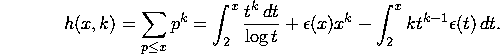
This first table is easily computed by noting that 3=0 in the coefficient ring.
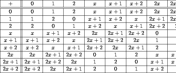
The multiplication table for T is easily computed if we remember
to replace ![]() by 1 whenever it appears in a product. We get:
by 1 whenever it appears in a product. We get:
Chapter 3, Problem 8.
![]()
where f(x) is this polynomial
![]()
The problem specification did not require a proof on why this works,
so I haven't provided one! In a nutshell, however, this algorithm
works because when x ;SPMgt; 0, ![]() . This means that when
x ;SPMgt; 0, the function is increasing, and hence we can rely on the
fact that, if f(a) ;SPMlt; n, then f(x) ;SPMlt; n for all
. This means that when
x ;SPMgt; 0, the function is increasing, and hence we can rely on the
fact that, if f(a) ;SPMlt; n, then f(x) ;SPMlt; n for all ![]() .
Similarly, if f(a) ;SPMgt; n, then f(x) ;SPMgt; n for all
.
Similarly, if f(a) ;SPMgt; n, then f(x) ;SPMgt; n for all ![]() . This
allows us to use a binary search to find the solution.
. This
allows us to use a binary search to find the solution.

This algorithm, in the worst case, is clearly ![]() , since
all it does is start with a search range of [0,n], and then it
uses a binary search to repeatedly half the range until it either
finds an x such that f(x) = n or it reduces the search range to
a single integer. Everything outside of the while loop in the program
will run in constant time.
The
, since
all it does is start with a search range of [0,n], and then it
uses a binary search to repeatedly half the range until it either
finds an x such that f(x) = n or it reduces the search range to
a single integer. Everything outside of the while loop in the program
will run in constant time.
The ![]() represents the worst case number
of calls to the function f, which I am assuming also runs in a constant
amount of time.
represents the worst case number
of calls to the function f, which I am assuming also runs in a constant
amount of time.
(************************************************************************
 Function DiophantineSolve takes as parameters a function f and an
   integer n, and returns either a non-negative integer x such that
   f(x) = n or -1 if no such non-negative integer exists.
************************************************************************)

DiophantineSolve[f_, n_] := Module[{},

    (* Set the range of integers in which we will find our answer *)
    rbegin = 0;
    rend = n;

    (* Choose our initial guess *)
    index = Floor[(rend+rbegin)/2];
    val = f[index];

    (* Search until we find an answer or run out of integers *)
    While[(rbegin != rend)&&(val != n),

        (* If the search range was of length 1, make it length 0 *)
        If[(rend-rbegin) == 1, rbegin = rend,
            If[ val > n, rend = index - 1, rbegin = index + 1]
        ];
        index = Floor[(rend+rbegin)/2];
        val = f[index];
    ];

    (* Set -1 as the return value if no answer was found *)
    If[ val != n, index = -1];
    index
]
(* Here we define f *)
f[x_] := 14x^17 + 99x^7 + 3x^2 + 94

(* Now we can solve part C on the homework *)
DiophantineSolve[f, 33110401974639861466556783753600023154051803888587048939300]
The Mathematica function found the solution:
![]()